The article Performance of machine learning classification models of autism using resting-state fMRI is contingent on sample heterogeneity (Maya A. Reiter, Afrooz Jahedi, A. R. Jac Fredo, Inna Fishman, Barbara Bailey, Ralph-Axel Müller, Springer Nature 2020) was chosen because it shows potential applications of machine learning in fMRI data analysis. Unsupervised machine learning has been widely used to study the brain connectome (an example is ICA), although in this article supervised learning was used and the authors showed that this approach is capable of producing better results.

The aim of this review is to give a general overview on machine learning and fMRI. Proteomics and fMRI data analysis share many issues like a huge amount of raw data and the necessity of new algorithms able to handle them. To do so machine learning may be a useful approach, both in proteomics and in neuroimaging.

Introduction

MRI and fMRI theory

Magnetic resonance imaging (MRI) is a widely used technique to acquire high quality images of internal tissues. Its main advantages are: it is not invasive, the magnetic field used is harmless and allows to visualize soft tissues, especially those rich in water or fatty acids.
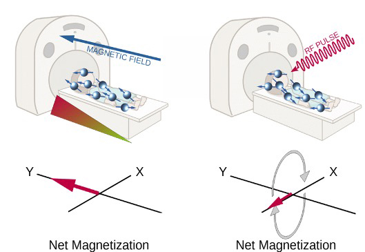
Images are acquired thanks to hydrogen atoms’ magnetic properties: each hydrogen nucleus is positively charged and since it is constantly spinning it creates a small magnetic field around itself. In normal conditions the aforementioned magnetic field is not detectable, since every field has a random direction. But when atoms are immersed in an external magnetic field they will align along its direction [figure A, left]. In these conditions atoms do not remain still and continue to wobble, causing their magnetic field to wobble as well. The frequency of such wobbling is called Larmor frequency and depends on the strength of the external magnetic field. At this point the scanner emits a radiofrequency pulse at the same frequency as Larmor’s one and this cause atoms to spin in phase and their net magnetization (the small magnetic field created by the sum of all atoms’ one) will then turn 90° and will rotate along the X axis [figure A, right]. This is the signal that is recorded by the machine, then when the radiofrequency pulse ceases this signal is gradually lost. The time required to lose this signal will be translated then into darker or brighter areas in the resulting images. Generally speaking, hydrogen atoms that are tightly packed together (like in fatty acids chains) will lose phase faster as well as atoms that are part of molecules that are freely to move in the tissue (like watery tissues).

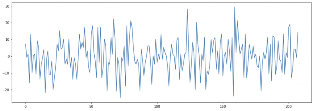
Functional magnetic resonance imaging (fMRI) uses the same principle, but instead of acquiring a single high resolution image it is used to obtain several images across a time interval to describe changes of magnetic properties in the studied tissue, in particular neuronal tissue. Haemoglobin when is not oxygenated can modulate the net magnetization, increasing the magnetic signal recorded by the scanner. Such property is used to describe where neuronal activity happens: when a brain region activates it signals to arteries to increase the blood flow to provide more nutrients and oxygen; at the same time some oxygenated haemoglobin spills into the venous system and this reduces the signal recorded and it is translated into brain activity in the specific region. In figure B is possible to visualize the signal recorded in one single voxel. The data is then “cleaned” removing the noise and eventual artefacts and then is analysed to study if oscillations are indeed caused by neural activity.

Connectivity analysis

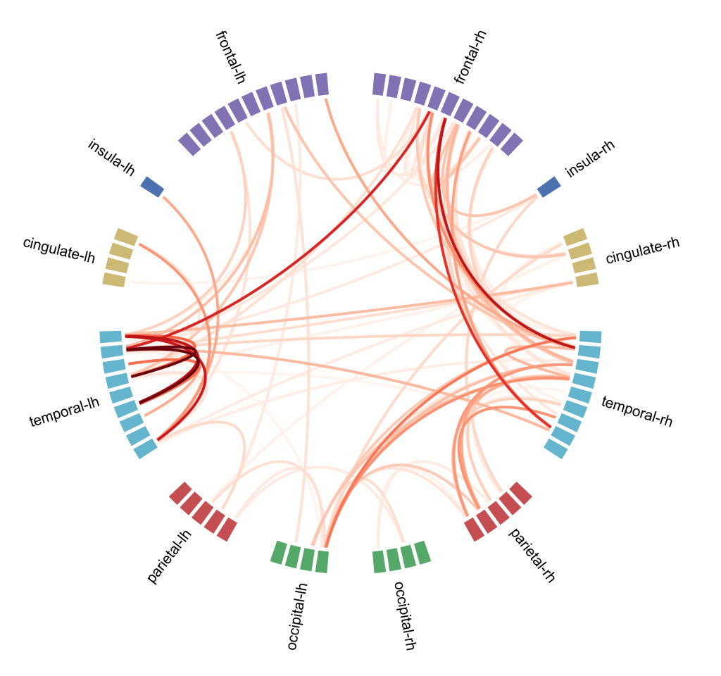
Connectivity analysis is a kind of analysis done on fMRI data, it is based on the assumption that if different brain regions have a similar pattern of activation they may be inter-connected and involved in similar cognitive functions. The aim is to create a map that shows connections between brain regions and how strong they are [figure C]. To do so one way is to use the independent component analysis (ICA): voxels are divided into components based on their activation pattern. ICA although is not the only machine learning approach that can be used, in particular supervised learning approaches seem to be more precise in describing the connectome.

Connectome analysis is used also to describe eventual abnormal patterns of brain activity that correlate with psychiatric disorders. Unfortunately it is quite difficult to study how psychiatric disorders affect patient’s brain activity: biological samples can be obtained only with post-mortem analysis and structural changes (that can be studied with MRI or PET scans) generally happen only at a very late stage of the disease. Currently connectome analysis showed some promising results in describing disorders at an early stage, in particular in this paper researchers used the connectome and machine learning approach to describe brain activity in autistic patients.

Machine learning

Since the first days of existence, learning has been an essential skill acquired by any living entity through experience, study, or being taught. With no exception, it is the same process among plants, animals, humans, and nowadays we can also teach machines to perform tasks.

Although machine learning is a new field, it has been improved and explored massively. Machine learning is a type of Artificial Intelligence that will enable machines to predict some outcomes by recognizing patterns in data rather than explicitly instructing them to do so.

Machine learning has a wide variety of applications not only in Proteomics but also in any field that has access to data, as former blog posts discussed the importance of data reproduction.

There are three different categories of Machine Learning, namely: Supervised learning, Unsupervised learning, and Reinforcement learning.

In this paper, researchers chose Random forest as their classifier which is a Supervised machine learning algorithm. Random forest is an Ensemble learning technique, where multiple learning algorithms are used in conjunction. So, instead of solving a problem with only one model, there are a group of models to solve the same problem by using a shuffled subset of the original data. The final result is the majority vote of model predictions.

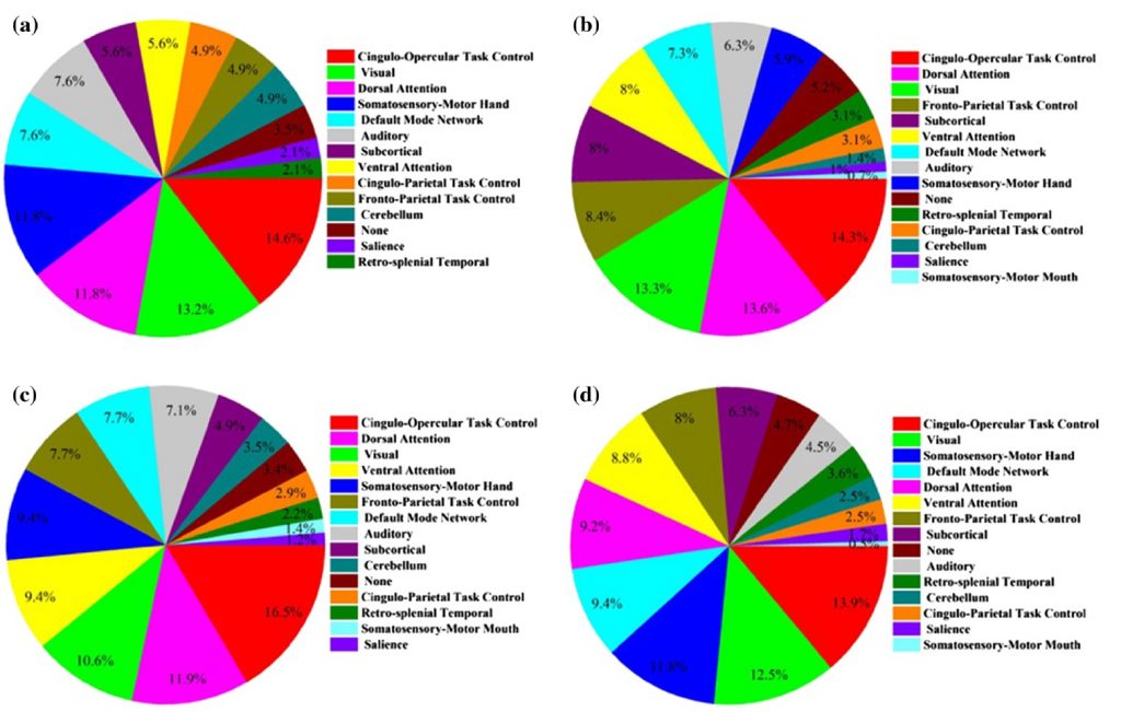
This paper mentions that random forest is superior to other ensemble methods in terms of accuracy, computational time, overfitting, and user interface to choose tree size. However, some other ensemble methods such as boosting can overcome random forest in case of accuracy and performance, but they also tend to be harder to tune. Random forest is used to build a diagnostic classifier in autism spectrum disorders (ASDs) samples with a focus on gender and symptom severity of 656 children and adolescents. The data was distinguished into four categories: all genders, only males, all genders with high severity range, and only males with high severity range. The classification accuracy of these categories was 62.5%, 65%, 70%, and 73.75%, respectively. Figure D demonstrates the portion of interest regions included in the classifier that achieved the peak classification accuracy from each of the brain networks for each sample group.

Conclusion

This paper aims to examine the impact of sample heterogeneity on the diagnostic classification of ASD. Reduced heterogeneity concerning gender and range of symptom severity was associated with improved performance of random forest classifiers. Random forest is implemented to build diagnostic classifiers in four ASD samples including a total of 656 participants. In conclusion, stratification by gender, symptom severity, age, cognitive ability, and other factors of variability may be critical in future efforts to pinpoint atypical brain features of ASDs. In particular the algorithm managed to select several brain regions that appears to be more interesting in describing differences between patients with mild and severe autism. Such differences are also in agreement with what has been studied in the past by psychologists and psychiatrists through cognitive tests.

There are although some limitations pointed out by the authors in the study: lack of enough data coming from female patients with ASD (common problem when studying autism since it is more frequent in males) and a relatively small number of samples used to describe the pathology, but they can be easily solved using wider and wider sample cohorts.